Hybrid dynamical systems with non-linear dynamics are one of the most general modeling tools for representing robotic systems, especially contact-rich systems. However, providing guarantees regarding the safety or performance of such hybrid systems can still prove to be a challenging problem because it requires simultaneous reasoning about continuous state evolution and discrete mode switching. In this work, we address this problem by extending classical Hamilton-Jacobi (HJ) reachability analysis, a formal verification method for continuous non-linear dynamics in the presence of bounded inputs and disturbances, to hybrid dynamical systems. Our framework can compute reachable sets for hybrid systems consisting of multiple discrete modes, each with its own set of non-linear continuous dynamics, discrete transitions that can be directly commanded or forced by a discrete control input, while still accounting for control bounds and adversarial disturbances in the state evolution. Along with the reachable set, the proposed framework also provides an optimal continuous and discrete controller to ensure system safety. We demonstrate our framework in simulation on an aircraft collision avoidance problem, as well as on a real-world testbed to solve the optimal mode planning problem for a quadruped with multiple gaits.

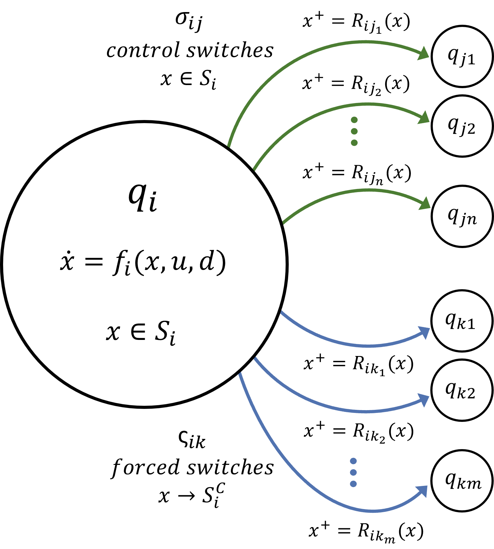
Consider a hybrid dynamical system with a finite set of discrete modes \(Q = \{q_1, q_2, ..., q_N\}\), connected through controlled or forced switches. We also refer to \(q_i\) as the discrete state of the system.

Let \(x \in X \subset \mathbb{R}^{n_x}\) be the continuous state of the system, \( u \in U \subset \mathbb{R}^{n_u}\) be the continuous control input, and \(d \in D \subset \mathbb{R}^{n_d}\) be the continuous disturbance in the system. In each discrete mode \(q_i \in Q\), the continuous state evolves according to the following dynamics:

\(\dot{x} = f_i(x, u, d)\)

\(q_i\) also has discrete control switches \(\sigma_{ij}\) that allow controlled transition into another discrete mode \(q_{j}\), where \(j \in \{j_1,j_2, ...,j_n\} \subset \{1, 2, ..., N\}\). Note that the number of discrete modes the system can transition into (that is, \(n\)) may vary across different \(q_i\). As \(x\) approaches \({S_i}^C\) (denoted \(x \to {S_i}^C\)), the system must take one of the forced control switches, \(\varsigma_{ik}\). This leads to a forced transition into another discrete modes \(q_{k}\) where \(k \in \{k_1,k_2,...,k_m\} \subset \{1, 2, ..., N\}\). Each discrete transition from \(q_i\) to \(q_j\), whether controlled or forced, might lead to a state reset \(x^+ = R_{ij}(x)\), where \(x\) is the state before the transition, \(x^+\) is the state after the transition.

Our key objective in this work is to compute the Backward Reachable Tube (BRT) of this hybrid dynamical system, defined as the set of initial discrete modes and continuous states \((x,q)\) of the system for which the agent acting optimally and under worst-case disturbances will eventually reach a target set \(\mathcal{L}\) within the time horizon \([t, T]\). Mathematically, the BRT is defined as:

\(\mathcal{V}(t)=\{(x_0, q_0): \forall d(\cdot), \exists u(\cdot), \sigma(\cdot), \varsigma(\cdot), \exists s \in [t, T], x(s) \in \mathcal{L}\}\)

where \(x(s)\) denotes the (continuous) state of the system at time \(s\), starting from state \(x_0\) and discrete mode \(q_0\) under continuous control profile \(u(\cdot)\), discrete control switch profile \(\sigma(\cdot)\), forced control switch profile \(\varsigma(\cdot)\), and disturbance \(d(\cdot)\). Along with the BRT, we are interested in finding the optimal discrete and continuous control inputs that steer the system to the target set. Conversely, if \(\mathcal{L}\) represents the set of undesirable states for the system (such as obstacles for a navigation robot), we are interested in computing the BRT with the role of control and disturbance switched, i.e., finding the set of initial states from which getting into \(\mathcal{L}\) is unavoidable, despite best control effort.

The core contribution of this work is Theorem I, an extension of the classical HJ reachability framework to hybrid dynamical systems with controlled and forced transitions, as well as state resets.

For a hybrid dynamical system, the value function \(V(x, q_i, t)\) that captures the BRT for an implicit target function \(l(x)\) is given by solving the following constrained VI:

If \(x \in S_i\):

\begin{multline} \min\{l(x)-V(x, q_i, t), \min_{\sigma_{ij}}V(R_{ij}(x), q_{j}, t) - V(x, q_i, t), D_{t}V(x, q_i, t)+ \max_{d \in D} \min_{u \in U} \nabla V(x, q_i, t)\cdot f_i(x,u,d)\} = 0, \end{multline}

and if \(x \in S_i^C\):

\begin{equation} \label{eqn:froced_transition_valfunc} V(x, q_i, t) =\min_{\varsigma_{ik}}V(R_{ik}(x), q_{k}, t) \end{equation}

With terminal time condition:

\begin{equation} V(x, q_i, T) = l(x) \end{equation}

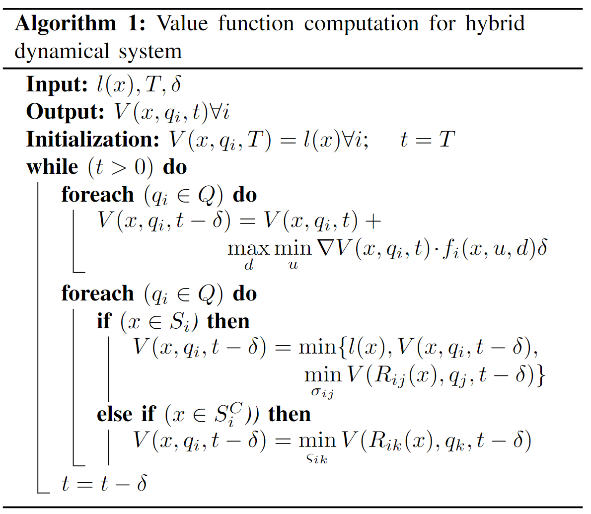
Numerical implementation: We now present an approximate numerical algorithm that can be used to calculate the value function in Theorem 1. It builds upon the value function calculation for the classical HJI-VI , which is solved using currently available level set methods [1]. Specifically, the value function is computed over a discretized state-space grid and propagated in time using a small timestep \(\delta\). After each propagation step, the value function is updated for all \((x,q)\) using Theorem I, until the time horizon \(T\) is reached.

To illustrate our approach, we consider very simplified, high-level dynamics for a robot quadruped moving in one dimension in a room with an obstacle (table). The robot goal is to reach the marked area on the other side of the table.

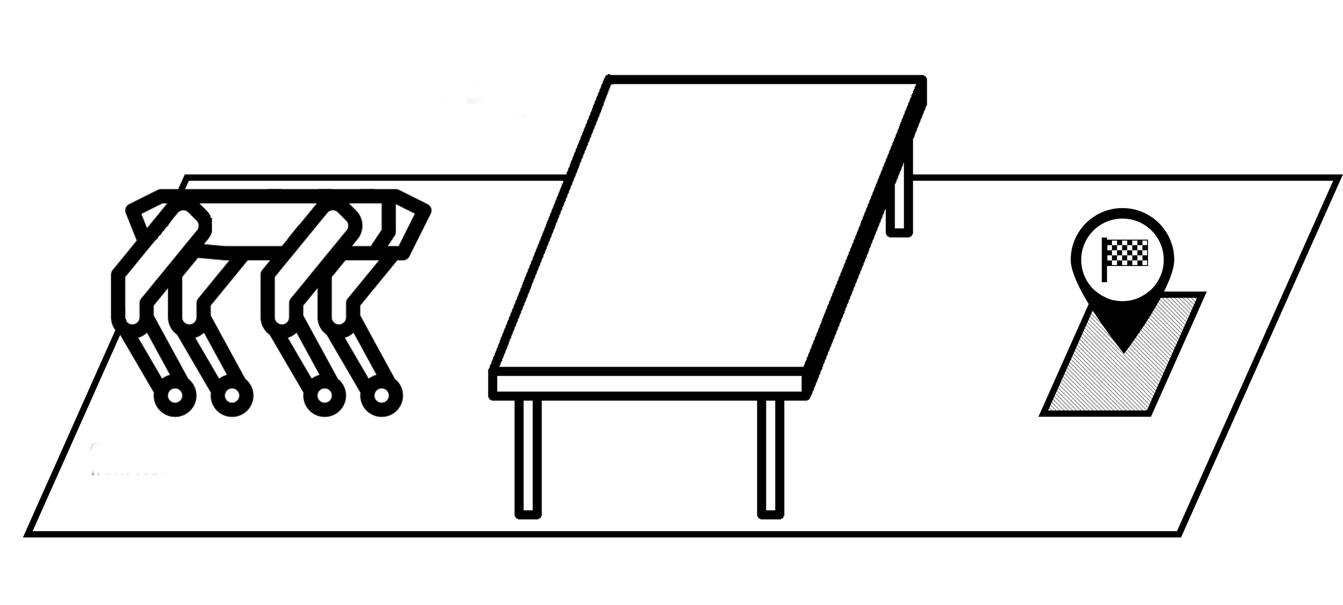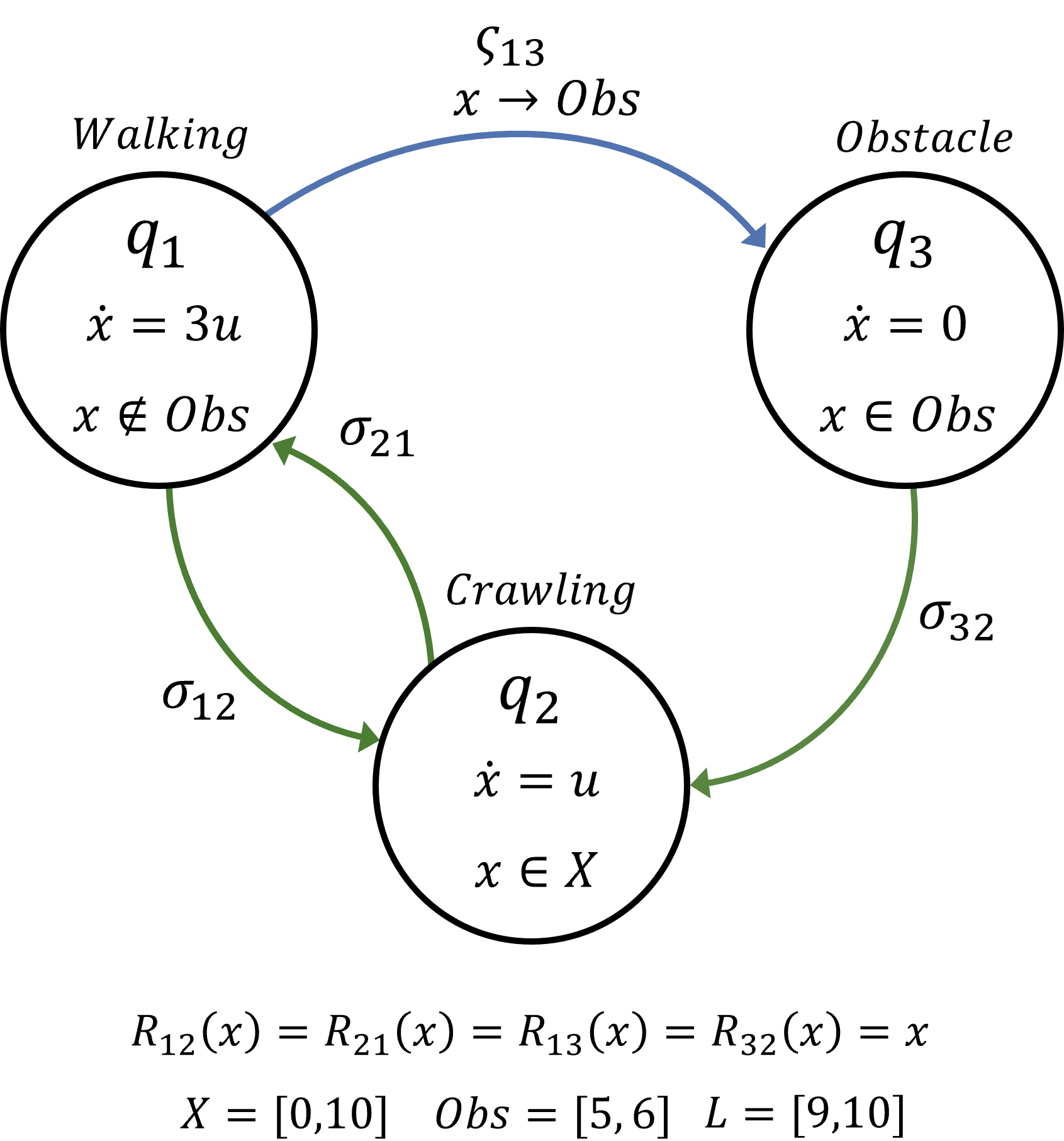
The hybrid system representation of this system is shown in the following diagram. Here, the continuous state \(x \in \mathbb{R}\) is the position of the robot and \(q_i\) with \(i \in \{1,2,3\}\) are the discrete modes of the system. \(u \in [0,1]\) is the continuous control of the system. The target set is given as the set of positions \(9 \leq x \leq 10\). In this example, \(q_1\) represents a walking gait, \(q_3\) represents frozen dynamics when the walking robot comes in contact with the table obstacle, and \(q_2\) is a crawling gait that allows the robot to move under the table but at a slower rate compared to walking.

The BRT for this example corresponds to all the combinations of continuous states and discrete modes \((x,q)\) from which the quadruped can reach the target set within a \(5\) second time horizon. Computing it using the classical Hamilton-Jacobi formulation with no optimal discrete mode switches gives the following results:

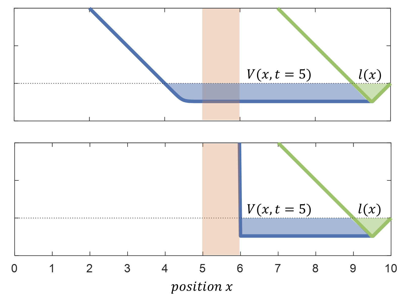
(Top) Value function for crawling gait mode. (Bottom) Value function for walking gait mode. Obstacle is shown in shaded red. Blue shade shows BRT as the subzero level of the value function. Green shade shows target set as the subzero level of \(l(x)\).

For the crawling gait it can be observed that the BRT (the blue shaded area) propagates through the obstacle and the BRT includes \(x=4m\) because the system can move at \(1m/s\) reaching the boundary of the target in exactly \(5s\). For the walking wait, even though the system is allowed to move faster, the BRT stops at the boundary of the obstacle as the walking gait gets stuck, so only states that start from the right side of the obstacle can reach the target set.

We now apply the proposed method to compute the BRT. To implement Algorithm 1, we use a modified version of helperOC library and the level set toolbox[1], both of which are used to solve classical HJI-VI. We use a grid of 301 points over the \(x\) dimension for each of the 3 discrete operation modes. The resulting BRTs are the following:

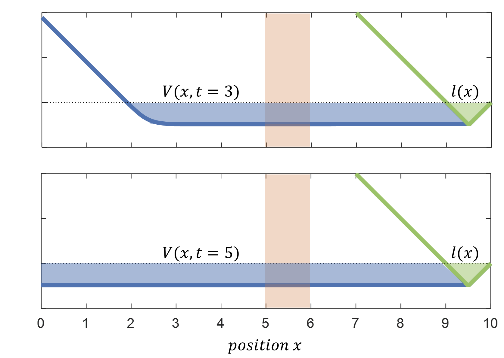
Value functions for states starting in a walking gait for a \(3\) and \(5\) seconds time horizon. Area within the obstacle is shown in shaded red. Blue shade shows BRT as the subzero level of the value function. Green shade shows the target set as the subzero level of the implicit target function \(l(x)\).

The intuitive solution for the optimal decision-making in this scenario is to use the walking gait everywhere except in the obstacle area. The fast walking gait allows the system to reach the target quicker, while crawling allows to expand the reachable states beyond the obstacle. The computed solution using our algorithm indeed aligns with this intuition. For example, if we consider the top value function for the 3-second time horizon, we can observe that the limit of the BRT is \(7m\) away from the target set, which coincides with the intuitive solution of walking for \(1s\) covering \(3m\), then crawling under the table for \(1s\) covering its \(1m\) width, to finally go back to walking for \(1s\) covering other \(3m\). The bottom value function shows the BRT corresponding to a \(5s\) time horizon. Compared to the previous classical attempt, where the BRT stopped growing beyond the obstacle boundary, we can see how the proposed algorithm can optimally leverage discrete transitions along with continuous control to reach the target set from a wider set of initial states.

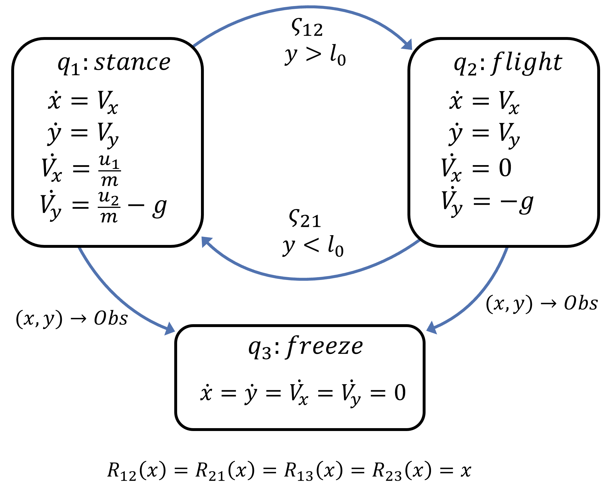
As a more challenging case study, we now consider a planar one-legged jumping robot that wants to reach a goal area on top of a raised platform. The center of mass dynamics of the jumper robot are shown in the following diagram. The robot has two main operation modes: a stance mode and a flight mode. The stance mode is active when the leg is in contact with the ground, which allows the leg to exert force and accelerate in xy directions. The flight mode is activated when the leg is no longer in contact with the ground, which is modeled as an unactuated ballistic flight. Additionally, we consider a freeze mode that will permanently halt the dynamics if the center of mass of the robot collides with the terrain; this modeling allows us to obtain the characteristic of a reach-avoid scenario while only doing reach calculations, since any trajectory that goes through the terrain will be frozen and excluded of the reach BRT as it will never reach the target set.

Hybrid formulation for the planar jumping robot.

In this system, the continuous state is given by \([x,y,V_x,V_y]^T\), representing both positions and velocities in the \(xy\) plane. Here \(u_1\) and \(u_2\) are the force inputs in the \(x\) and \(y\) directions, both with an actuation range of \(0-30 N\). \(l_0=0.5m\) is the length of the robot leg, \(m=1kg\) is the mass of the robot, and \(g\) is the acceleration due to gravity. The target set is a circular area in the \(xy\) plane on top of a raised platform, which is considered to be part of the terrain along with the ground; the objective here is to find all the initial states of the robot in the stance mode from which a successful jump into the target set is guaranteed without colliding with the platform.

In the following clip we show results for this example. There the blue BRT shows all the resting stance states that guarantee reaching the target without colliding into the obstacle. We present a trajectory and slow down at the mode transition to see how it moves between different slices of the BRT. One interesting highlight of this example is how the robot builds momentum to optimally use the forced transition. These behaviors are not hard-coded in the system, they automatically emerge out of the reachability analysis.

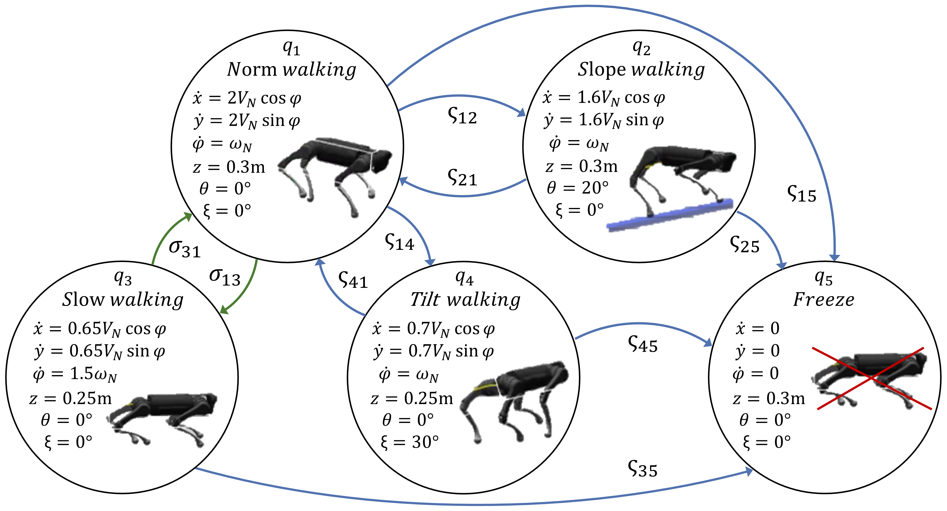
We next apply our method for task-based, high-level mode planning on a real-world quadruped robot, to reach a goal position in a terrain consisting of various obstacles. The quadruped has different walking modes, such as normal walking, walking on a slope, etc., each of which is modeled as a discrete mode in the hybrid system as shown in the following diagram:

Within each discrete mode, we use simplified continuous dynamics to describe center-of-mass evolution:

\begin{equation*} \dot{x} =k_x V_{N} \sin \varphi + d_x; \quad \dot{y} =k_y V_{N} \cos \varphi + d_y; \quad \dot{\varphi} =k_{\omega} \omega_{N}, \end{equation*}

where the state \([x,y,\varphi]^T\) represent the \(xy\) position and heading angle of the robot. \(V_{N} = 0.25m/s\) is the fixed (normalized) linear velocity and \(\omega_{N} \in [-0.5, 0.5] rad/s\) is the angular velocity control. \(k_x\), \(k_y\), and \(k_{\omega}\) are velocity gains for different operation modes. \(d_x\) and \(d_y\) are bounded disturbances on \(xy\) velocity. Also, we use discrete state \([z,\theta,\xi]^T\) to set the body's height, pitch, and roll angle in different operation modes for overcoming various obstacles.

Each operation mode matches a specific obstacle or terrain in the testing area. The quadruped begins in mode \(q_1\) for fast walking. If the robot reaches the boundary of the slope area, the system will be forced to switch to mode \(q_2\) with a \(20^{\circ}\) body pitch angle for slope climbing. At some time, the control may switch to mode \(q_3\) to walk slowly with a lower body height, this allows the robot to make a narrow turn or crawl under obstacles. If the robot encounters a tilted obstacle, the system will go through a forced switch into mode \(q_4\) to walk with a tilted body. Whenever the robot touches a ground obstacle, the system will stay in mode \(q_5\) permanently with frozen dynamics. The quadruped needs to reason about optimally switching between these different walking modes in order to reach its goal area (the area marked as the pink cylinder in following videos) as quickly as possible without colliding with any obstacles. BRT for this experiment is calculated on a \([x,y,\varphi]\) grid of \([40,40,72]\) points, over a time horizon of \(t=45s\). Having the BRT, we can acquire optimal velocity control, operation mode, and the desired discrete body states at each time. The quadruped is equipped with an Intel T265 tracking camera, allowing it to estimate its global state via visual-inertial odometry. The high-level optimal velocity control and discrete body states provided by our framework are then tracked by a low-level MPC controller that uses the centroidal dynamics of the quadruped.

Our first experiment result is shown in the accompanying video. In our environment setup, the optimal (fastest) route to reach the target is via leveraging the slope on the right. Specifically, the robot remains in the normal walking mode and switches to the slope walking mode once near the slope. When the robot approaches the end of the slope, it needs to make a tight left turn to avoid a collision with the wall ahead. Our framework is able to recognize that and makes a transition to the slow walking mode to allow for a tighter turn. Once the turn is complete, the robot goes back in the faster walking mode.

In our second experiment, we put some papers on the slope, making it more slippery. This is encoded by adding a higher disturbance in the slope mode \(q_2\). The new BRT makes the slope path infeasible and hence the robot needs to reach the target via the (slower) ground route. Once again, apart from selecting a new safe route, the proposed framework is able to switch between different walking modes along the route to handle tight turns and slanted obstacles, as shown by the activation of the tilt walking mode.

Finally, to test the closed-loop robustness of our method, we add human disturbance in the ground route experiment. The robot is kicked and dragged by a human during the locomotion process. Specifically, the robot was dragged to face backward, forcing it near the tilted obstacle. However, the reachability controller is able to ensure safety by reactivating the tilt walking mode, demonstrating that the proposed framework is able to reason about both closed-loop continuous and discrete control inputs. Nevertheless, it should be emphasized that the presented algorithm does not solve the entirety of legged locomotion planning, but rather only provides the top level of a hierarchical planning architecture that typically include a robust footstep planner, a wholebody controller, and reliable state estimation.

We present an extension of the classical HJ reachability framework to hybrid dynamical systems with controlled and forced transitions, and state resets. Along with the BRT, the proposed framework provides optimal continuous and discrete control inputs for the hybrid system. Simulation studies and hardware experiments demonstrate the proposed method, both to reach goal areas and in maintaining safety. Our work opens up several exciting future research directions. First, we rely on grid-based numerical methods to compute the BRT, whose computational complexity scales exponentially with the number of continuous states, limiting a direct use of our framework to relatively low-dimensional systems. We will explore recent advances in learning-based methods to solve HJI-VI to overcome this challenge. Another interesting direction would be to extend our framework to the cases involving uncertainty in the transition surface \(S_i\) or where controlled switches have different transition surfaces. Finally, we will apply our framework on a broader range of robotics applications and systems.

[1] I. Mitchell, “A toolbox of level set methods,” http://www.cs.ubc.ca/mitchell/ToolboxLS/toolboxLS. pdf, Tech. Rep. TR-2004-09, 2004.